Heisenberg vs Schrodinger picture

See also states and observables.

Schrodinger picture in QM

Remember that to solve a Quantum Mechanics problem we solve the Schrodinger equation

with initial condition $f(x)$.

When we want to observe the system or make a prediction, at a desired time $t$, "we apply" a desired observable $\hat{Q}$ to $\Psi(x,t)$, obtaining a real value:

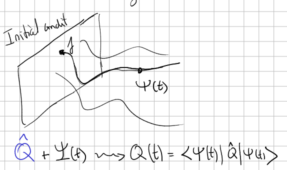
Schrodinger picture in CM

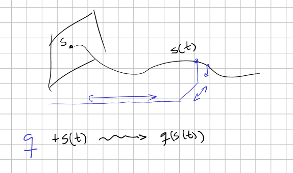
To compare this with Classical Mechanics, for example a particle in a potential, you have to think of the states $s$ of the particle as living in an abstract set $S$ (something like the "Configurations of the Real World") and observables like "standardized procedures" to obtain a numerical value from a state. For example, the observable "position" $q$ would be a system of sticks or rods, independent of the state of the particle and independent of time, in the same way that $\hat{Q}$ is independent of $\Psi$ and $t$.

When we write $q(t)$ we indeed mean the composition of maps

Observe that these standard procedures are independent of time: we have established beforehand how are we going to take measures with our rods...

The key difference with QM is that in CM, the authentic state $s$ is not a mathematical object unlike the wavefunction $\Psi$ of QM. So in CM we are forced to write the differential equations in terms of the composed maps $q\circ s$, instead of with the states itself.

But there is a trick. We usually assume the existence of observables that let us create a bijection between the set $S$ and a numerical set, for example $\mathbb R^2$ in the standard example of Hamiltonian mechanics:

So you identify the states $s$ with the pairs $s\equiv (q,p)$ and this way you can write differential equations directly for the states:

with $X_H$ the corresponding Hamiltonian vector field. This would be Schrodinger equation (1) for CM.

And now, you have two distinguished observables (standard procedures) $\pi_1,\pi_2$, the projections over the first and second coordinates. Indeed, all the "standardized procedures" get transformed under this identification into other "math operations" with $q$ and $p$. Now, you solve problems in a totally analogous way to Schrodinger picture: evolve the state $s_0$ with the ODE above to a time $t$ and then use a observable (for example $q=\pi_1$) to obtain the prediction $Q(t)=\pi_1(s(t))$. So far, so good.

Heisenberg picture in CM

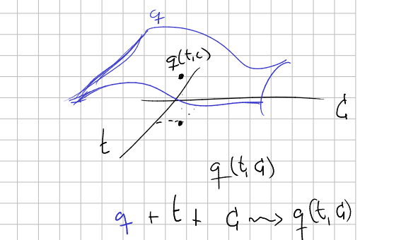
The use (and abuse) we do of $q(t):=q(s(t)), p(t):=p(s(t)),...$ makes us think that observables $q,p,...$ are other kind of entities. They are considered maps associating a numerical value to a time $t$ together with an initial condition $C$, and satisfying some differential equations.

Observables constitute a commutative c-star algebra.

And we have that the evolution of one of them is given by the equation

where $H$ is the Hamiltonian and $\{.,.\}$ the Poisson bracket. This is related to the flow of observables in CM.

Heisenberg picture in QM

This different approach to observables like smooth functions let us think of them as elements of an algebra, which is commutative. For different reasons (see Why did physics go quantum) we suspect that the algebra of observables should be a noncommutative c-star algebra. I guess this is related to Noncommutative Geometry. So instead of time dependent functions of the state space, we take time dependent operators in the wavefunction space.

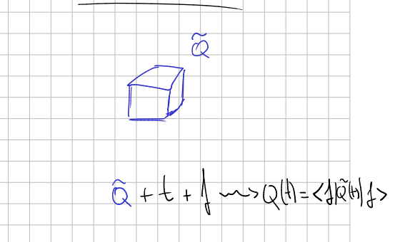
These operators, once they are known, are waiting for us to provided a time $t$ and an initial condition $f$ to yield a value, as in Heisenberg picture for CM, but now with $\langle f |\tilde{Q}(t)| f \rangle$.

Mathematically, the relation between Schrodinger and Heisenberg picture comes as follows. A formal solution of equation (1) is

indeed this is nothing but other way to write (1).

Now, for every observable $\hat{Q}$ we define the time-dependent operator

In order to make predictions it is clear that (2) is substituted by

Observe that $\tilde{Q}$ satisfies

since

and since $e^{-i\frac{\hat{H}}{\hbar}t}$ commutes with $\hat{H}$

as desired.

Observe that equation (6) correspond to equation (4).

Worked example (to be corrected and adapted)

Let's solve for the average position of a free particle described by the given wave function in the Heisenberg picture.

1. Time Evolution of the Position Operator in the Heisenberg Picture

For a unit mass free particle, the Hamiltonian is given by:

where $\hat{p}$ is the momentum operator.

The Heisenberg equation of motion for the position operator $\hat{x}_H$ is:

In CM this corresponds to $H=\dfrac{1}{2}p^2$, and the equation of motion would be

Using the commutation relation between the position and momentum operators:

$$ [\hat{x}, \hat{p}] = i\hbar $$

The commutator between $\hat{H}$ and $\hat{x}_H(t)$ is:

$$ [\hat{H}, \hat{x}_H(t)] = \frac{1}{2m} [\hat{p}^2, \hat{x}_H(t)] $$

$$ = \frac{1}{2m} (\hat{p} \hat{p} \hat{x}_H(t) - \hat{x}_H(t) \hat{p} \hat{p}) $$

Given that $[\hat{p}, \hat{x}_H(t)] = -i\hbar$, and using $\hat{p} [\hat{p}, \hat{x}_H(t)] = -i\hbar \hat{p}$, we get:

$$ [\hat{H}, \hat{x}_H(t)] = \frac{\hat{p}}{m} $$

Now, plugging this into the Heisenberg equation, we get:

$$ \frac{d\hat{x}_H(t)}{dt} = \frac{\hat{p}}{m} $$

Integrating this (and noting that the initial position operator is just $\hat{x}$), we find:

$$ \hat{x}_H(t) = \hat{x} + \frac{\hat{p}t}{m} $$

2. Computing the Expectation Value at Time $t = 3$

$$ \langle x(3) \rangle = \langle f(x) | \hat{x}_H(3) | f(x) \rangle $$

$$ = \langle f(x) | (\hat{x} + 3\hat{p}) | f(x) \rangle $$

$$ = \langle f(x) | \hat{x} | f(x) \rangle + 3 \langle f(x) | \hat{p} | f(x) \rangle $$

Given $f(x) = (2/\pi)^{1/4} e^{ix/\hbar} e^{-x^2}$:

$$ \langle f(x) | \hat{x} | f(x) \rangle = \int dx f^*(x) x f(x) $$

$$ \langle f(x) | \hat{p} | f(x) \rangle = -i\hbar \int dx f^*(x) \frac{df(x)}{dx} $$

Both of these integrals can be computed directly.

$$ \langle f(x) | \hat{x} | f(x) \rangle $$ yields $0$ due to the symmetrical nature of the state.

$$ \langle f(x) | \hat{p} | f(x) \rangle $$ yields $1$ based on the integral of the given wavefunction and its derivative.

Thus, the average position at $t = 3$ is:

$$ \langle x(3) \rangle = 0 + 3(1) = 3 $$

This result is as expected since the free particle's wave packet moves to the right with an average momentum of $\hbar$, resulting in an average displacement of $3$ units over the time $t = 3$.

________________________________________

________________________________________

________________________________________

Author of the notes: Antonio J. Pan-Collantes

antonio.pan@uca.es